
Introduction
Background
Hello! I am Kinon, an Indonesian Software Engineer at ID Platform of Money Forward’s Business Platform Development. I worked fullstack in this team for about 6 months. I would like to share one branch of one of my hobbies that I actually started during my university, which is Problem Setting in Competitive Programming. I will abbreviate Competitive Programming as CP.
As you may have noticed, this blog has very similar title and topic to one of Money Forward’s previous blog I Tried Kotlin for CP. It was written by my colleague Wibi, who actually almost always teamed up with me during our university years in competitions. His blog has become an inspiration to me creating this in an effort to extend the topic further and unravel more things about CP that may interest the general public, hence I want to pay my tributes.
CP Problem Setting
You can define CP in many ways, but to me it is developing a solution, data structure, or algorithm, spending as little time as possible compared to other competitors, such that the program:
- Runs faster than the maximum time limit given
- Use less than the maximum memory limit given
- Still gives correct answers to the problem
For all of the possible cases that can be given as long as it satisfies the test case contraints given in the problem. From here onwards I will abbreviate test case as TC.
I think the three listed points above differentiate those who are already familiar with CP and those who are not. The ones practicing this field have these facts already ingrained in their minds whenever they solve a problem. However in my experience, many people including the ones familiar, still do not have the part after the third point as a given yet. Many people often do not realize that the algorithm they developed did not satisfy one of the time constraint, or space constraint, when being faced by edge cases or special cases specifically constructed to counter that approach.
Many people dealing with algorithms are probably familiar with big-O notations as well, that can be applied to time complexity and space complexity. It is a notation to show how much the growth rate of the time and space needed in that program is, over the size of the problem. My experience with this is, they often take the big-O notation of well known algorithm they used in their solution for granted. Often using the average complexity without considering how the worst case interact with other parts of the solution, and use it as a big-O which is false.
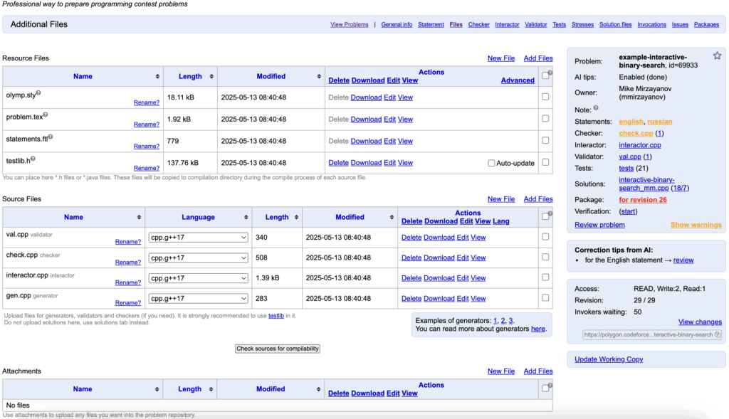
According to my experience, there are 8 main components needed for problem settings. As shown in the picture above, it is displaying most files needed in Polygon, a problem setting platform for CodeForces. The problem used is “example interactive binary search”, a public example by Mike Mirzayanov, the creator of CodeForces. These main components are listed as follows.
1. Problem statement
This is the only component that will be visible to the solver. The statement contains the problem description itself (how to get the correct output from the input), constraints (time, space, input variables), and sample TCs (how the input is provided and how the program should output).
2. Jury’s solution
Of course there should be a valid solution that actually solves the problem satisfying all constraints. When being executed using the TCs, it is recommended that the time and space used are no more than half of the time and memory limit stated in the problem.
3. TC generator(s) and manual TCs if any
Sample TC are an example of manual TC, since it is constructed by hand to make the reader easily follow, get familiar with, or simulate the problem themselves. But it will be pretty tiresome if all testcases are crafted by hand, hence it is easier if it is generated from the Jury’s solution. There can be many generators, each targeting to filter out different algorithms or approaches. When combined they will produce a set of TCs that hopefully accepts only intended solutions.
4. Validator (recommended)
A file to run for each TC, making sure that each satisfies the constraint provided in the problem statement. The use of this file is more needed if there are some not-so-simple constraints, like in graphs or matrices satisfying special rules, instead of simple constraints like only making sure a variable’s value is inside an interval.
5. Alternate solution (recommended)
Although a problem can exist without one, it is highly recommended as a sanity check that a solution, preferably written in different style, approach, or even person, be used right on the TCs generated by the Jury’s Solution. It has to get an “Accepted” verdict.
6. Other solution that is not meant to pass (optional)
Developing solutions that are meant to fail can be easily paired with the corresponding TC generators that are specifically designed to make them failed. This also make the development more structured and have way less accidents along the way, in my experience.
7. Checker (optional)
Problems that have multiple solutions and encourage solvers to output any of the solutions, need a checker component in its problem setting. A checker component is a file that receives the solver’s program’s output as their input, and outputs a verdict whether it is “Accepted” or “Wrong Answer”.
8. Communicator (optional)
There is a genre in CP problems called interactive problem. To solve it, we basically need to make a program that continuously receiving inputs, then outputs, then back to receiving inputs, in that order until some final condition is reached. To compose this kind of problem, we need to develop a communicator file that will act as the name suggest, communicate back and forth to the solver’s program.
I have also worked on Problem Setting without using Polygon as a platform. Instead I use my local machine to generate test cases using TCframe as a framework. Typically for each problem composed using this framework, there is one generator file spec.cpp that contains all generation algorithms, so it can be lengthy in the end. For example, this tutorial about creating simple tree graph TCs is already quite lengthy, even though it is the basics of setting a problem that involves graphs in it. Some of its observation will be relevant in the next section.
Composing a Meta Defining Problem for Competitive Programmers
Now I am going to present a problem as a case study for CP problem setting. The reason I chose the problem is that it is related to some (not only one) well established algorithm used in this field. In my opinion, familiarity with these kinds of algorithms is the difference between an avid Competitive Programmers and those who are not. I will not reveal the solution until right before the end of this section, to walk us through solving the problem. The problem is a slightly harder modification of Path Queries, and it goes as follows.
Problem Statement
Time Limit: 2.0s, Memory Limit: 524MB
You are given a rooted tree consisting of n nodes. A tree is a graph (a structure of node and edges that connects two nodes) of n-1 edges so that each pair of node is reachable. The nodes are numbered 1,2,…,n, and node 1 is the root. Each node has a value.
Your task is to process following types of queries:
- Change the value of node s to x
- Calculate the sum of values on the path from node a to node b
Input
The first input line contains two integers n and q: the number of nodes and queries. The nodes are numbered 1,2,…,n.
The next line has n integers v1,v2,…,vn: the value of each node.
Then there are n-1 lines describing the edges. Each line contains two integers a and b: there is an edge between nodes a and b.
Finally, there are q lines describing the queries. Each query is either of the form 1 s x or 2 a b.
Output
Print the answer to each query of type 2.
Constraints
- 1 ≤ n, q ≤ 106
- 1 ≤ a, b, s ≤ n
- 1 ≤ vi, x ≤ 109
Note: The well-established benchmark used in CP is that 1 second is equivalent to 108 primitive operations (addition, assignment, array access, etc).
Sample Test Case
Input
5 3
4 2 5 2 1
1 2
1 3
3 4
3 5
2 1 4
1 3 2
2 4 2
Output
11
10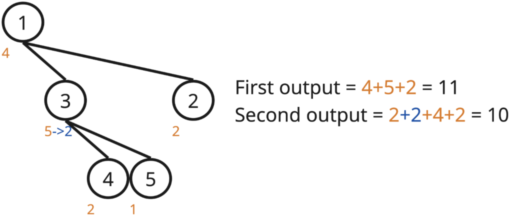
The Most Naive Solution
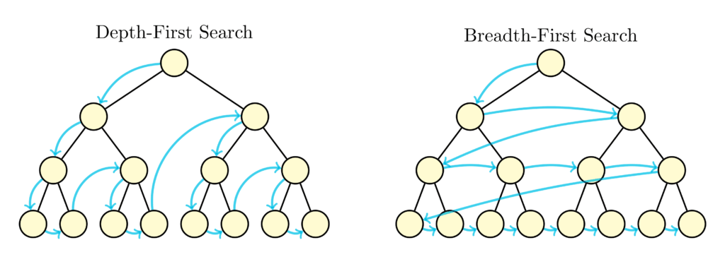
We can picture ourselves the sample test case to better understand the problem. Looking at the first query and the fact that it is a graph, the two most famous algorithm about pathfinding comes to mind: Depth First Search (DFS) and Breadth First Search (BFS).
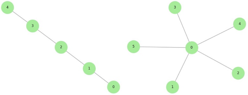
If we decide to use one of these in our solution, each type 2 query will have average O(n) time complexity which is bad enough since we will have O(nq) complexity at worst, way more than 108. Moreover problem setters can even include a testcase with a path and a star graph to test the limit of recursion call in DFS and queue size in BFS.
// Path Graph of n nodes 1..n
vector<int> path;
for(int i=0; i<n; i++) path.push_back(i+1);
shuffle(path.begin() /* +1 if assure depth n */, path.end());
vector<pair<int, int>> edges;
for(int i=1; i<n; i++) edges.push_back({path[i-1], path[i]});
shuffle(edges.begin(), edges.end());

// Star Graph of n nodes 1..n
vector<pair<int, int>> edges;
for(int i=1; i<n; i++)  edges.push_back(rnd.next(2)>0 ? {1, i+1} : {i+1, 1});
shuffle(edges.begin(), edges.end());
We might ask ourselves, is there a way to not search the path for every query? Can we already know which path to take for every pair of node {a, b}, since in a tree there is only one possible path anyway?
Use the Fact That the Graph is a Tree
Now let us call:
- Node 1 as the root of the tree
- A parent of node x is a node next to x that is directly on the path of x to root. It can be seen that every node except 1 has exactly one parent.
- A depth of node x is the distance to node 1, with the depth of node 1 being 0.
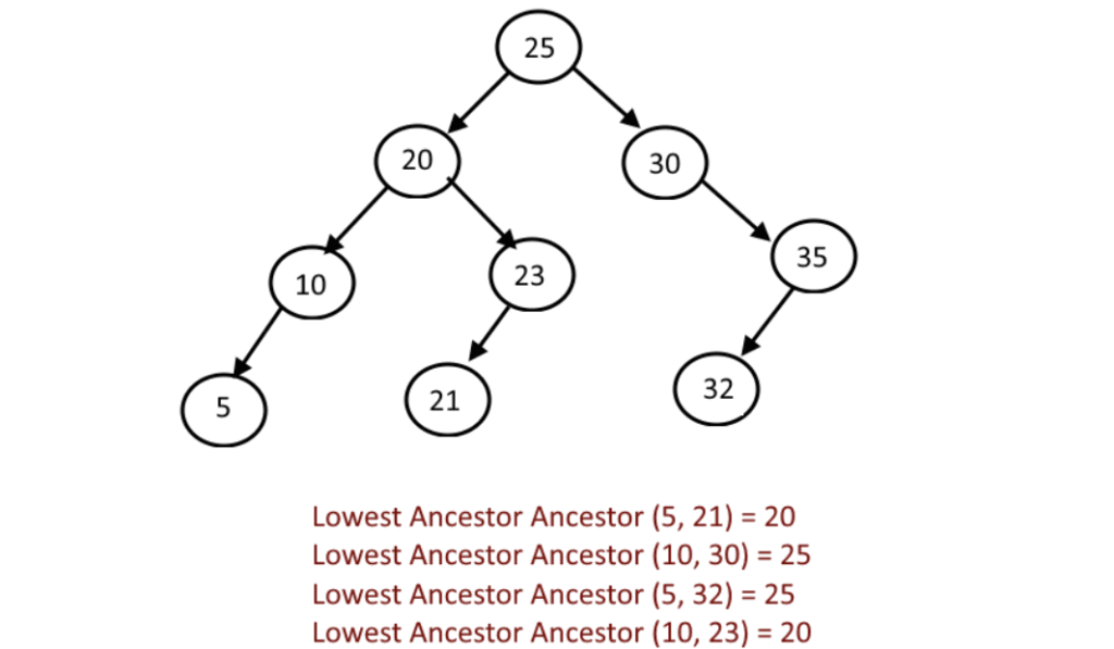
With this, we can easily traverse only the nodes directly inside the shortest path of a to b for every query. How?
- Keep track of two pointers, starting at a and b
- If the depth of the first pointer is higher than the depth of the second, move the first pointer to its parent. Otherwise move the second pointer to its parent.
- Eventually they both will coincide, making a complete path connecting a to b. This point is commonly called Lowest Common Ancestor (LCA).
Now even if they have lessen the average complexity from our naive solution by a lot, especially in the worst TCs, it still has O(dq) complexity with d being the tree’s max depth.
However it can be noted that this solution can pass most of the TCs if it is randomly generated. This is because randomly generated tree often has depth far lower than its node count. So for problem setters, it is important to provide cases where the generated tree is deep enough, O(n) depth for example. Make sure to also create TCs where the LCA of the queried node is far from the root node, as there may be solutions doing the opposite calculating from the shallow nodes to the deeper ones. Below is one way to generate a tree that satisfies this.
// Randomly generate tree with 99 nodes
// this will have average depth of around 10
int parent[100]
for(int i=2; i<100; i++) parent[i] = rnd.next(1,i-1)
// Use this tree as a skeleton, put other nodes between the skeleton node and its parent
vector<int> inbetween[100];
for(int i=100; i<=n; i++) inbetween[rnd.next(2,100)].push_back(i);
vector<pair<int, int>> edges;
for(int i=2; i<100; i++){
  shuffle(inbetween[i].begin(), inbetween[i].end);
  edges.push_back({parent[i], inbetween[i][0]})
  int sz = inbetween[i].size();
  for(int j=1; j<sz; j++)
    edges.push_back({inbetween[i][j-1], inbetween[i][j]})
  edges.push_back(inbetween[i][sz-1], i);
}
shuffle(edges.begin(), edges.end());
// Each edge from the skeleton becomes n/100 edges on average, making the expected depth is about n/10
// To increase the depth just decrease the skeleton
Binary Lifting
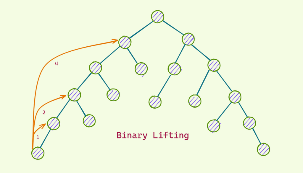
Now what if I tell you we can further improve our LCA finding algorithm to O(log(d)) instead of O(d)? Instead of only storing the direct parent of each node, why don’t we store log(d) values of parenti that represents 2i times the parent of said node. To clarify:
- parent1(x) is parent0(parent0(x))
- parent2(x) is parent1(parent1(x))
- and so on…
- We can calculate in log(d), for example parent-25-levels above x is parent4(parent2(parent0(x)))
- To find LCA of a and b we can first lift the deeper node to the same level, then iterate i from the greatest possible value to the lowest:
- If parenti(a) = parenti(b), do nothing
- Otherwise, move a to parenti(a) and b to parenti(b)
Another important information is to store, in each node, the sum of v of all nodes from that node to the root, instead of storing the node values itself. Lets call this new value in node x as sumToRoot(x). This way, the sum of all values in path a to b is equal to sumToRoot(a) – sumToRoot(LCA(a, b)) + sumToRoot(b) – sumToRoot(LCA(a, b)). This is a very simple O(1) formula.
Now we have found the general idea for the query part (type 2 in the problem), all that is left is to integrate it with the update part (type 1 in the problem). Because now we have to worry that since we store sumToRoot values, that means an update to a node x value affects sumToRoot of all node inside the subtree of x. For problem setters, I suggest you to add plenty of update queries on different nodes that “matters”, meaning is present in many queried path.
int maxDepth;
vector<int> nodesByDepth[maxDepth+1];
// assuming the nodes on the generated has been stored based on their depth
int type1Count, type2Count;
vector<pair<int, int>> type1Queries, type2Queries;
for(int i=0; i<type1Count; i++){
  // update the node half most shallow one, to affect many paths
  int depth = rnd.next(maxDepth/2);
  int size = nodesByDepth[depth].size();
  int node = nodesByDepth[depth][rnd.next(size)];
  type1Queries.push_back({node, rnd.next(maxValue)});
}
for(int i=0; i<type2Count; i++){
  // depth differs a lot
  // both nodes not close to root so the path is long
  int depth1 = rnd.next(maxDepth/3, maxDepth*2/3);
  int depth2 = rnd.next(maxDepth*2/3, maxDepth);
  int size1 = nodesByDepth[depth1].size();
  int size2 = nodesByDepth[depth2].size();
  int node1 = nodesByDepth[depth1][rnd.next(size1)];
  int node2 = nodesByDepth[depth2][rnd.next(size2)];
  // deeper node as first or last
  type2Queries.push_back(rnd.next(2)>0 ? {node1,node2} : {node2,node1});
}
Flattening the Tree
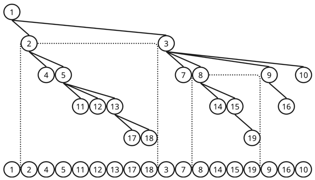
Another concept, a euler tour, is an order of nodes that is visited if we do a DFS from the root of the tree. Now the thing that blows my mind the first time I learned about it is, the subtree of node x (nodes that passes x if they want to traverse to root) is always displayed consecutively in the euler tour (for example the subtree of node 2 and the subtree of node 8 in the image above). This means that we can transform the tree to our new data structure, which is a simple array that we get the order from euler tour, and each of its value being sumToRoot(x).
This way we need a method of adding x to all value in the array in any index range a to b for the type 1 query. And recalling the value of the array in any index x at any point in time. This is what I called a “Point Update Range Query” problem. I do not want to dwell on this topic too deep, since both the solution and the TC generation can be discussed concisely.
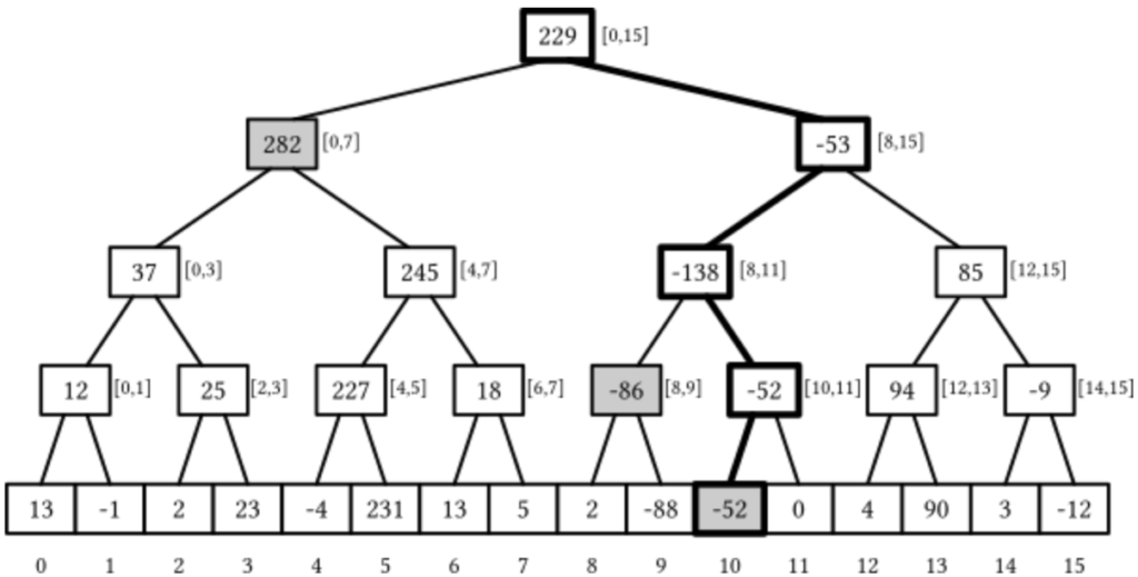
The infamous data structure segment tree can be used to make sure the update and query functionality of our data structure both be done in O(log(n)). For TC generation, make sure:
- Make sure to test both extremes of the number of query types. Meaning TC including many type 1 lesser type 2, or vice versa.
- To avoid passing a submitted program that do the range update iteratively, make sure to include many long ranges. Likewise, make sure to also include many short ranges in other TCs
- Make sure to shuffle the order of the type being queried, maximize the type switching! Why is this important? Because there may be a solution that rebuilds their entire data structure before every adjacent query, and/or bulk update their data for every adjacent updates.
int type1Count = 100, int type2Count = n-100
// or
int type1Count = n-100, int type2Count = 100
vector<pair<int, pair<int, int>>> queries;
for(int i=0; i<type1Count; i++){
  // ...
  // in the end push to queries instead
  queries.push_back({1, {/* ... */}});
}
for(int i=0; i<type2Count; i++){
  // ...
  // in the end push to queries instead
  queries.push_back({2, {/* ... */}});
}
shuffle(queries.begin(), queries.end());
Other Methods: Use Randomization
Until this point, we have made countermeasures for possible mistakes across each step of solving the problem using the intended solution. However there is a possibility that there is another solution that also solves the problem, satisfying time limit, memory limit, and correctness over all possible TCs satisfying the problem’s constraint. It may be that the problem setters did not realize this solution is viable, hence it is not touched by the intended and all alternate solutions. However the problem should still accept this solution, and provide a strong enough TCs in the hopes of that stress testing any kind of solution, generally speaking. Stress testing is making the program goes through TCs that push it to the maximum correctness (by maximizing calculations needed), memory, or time limit. TCs satisfy as a stress test if each of those aspect is tested in at least one TC.
Randomization is a great tool for this. By creating many TCs that we still do not know currently what kind of wrong solutions will each TC fails, it will exponentially shrink the probability of a wrong solution, to be accepted. These TCs can also fail an intended solution that has small mistakes, for example a slight error on a loop condition may get “Time Limit Exceeded” on a TC by chance, a bit of a typo can get “Wrong Answer”, wrong branch condition can get a “Runtime Error”, etc. A whole other generator that produces purely random TCs is almost a must-have in many kinds of problems!
In a way, aside from making another TC generator that is pure random, problem setters can also incorporate a bit of randomization to the previous well-defined TCs. However we need to keep in mind that, as powerful as randomization can be, we cannot let it taint the true goal of our previous TCs. For example if we want to create a tree deep enough or at least O(n) we do not randomize the tree generation because it will produce a shallow tree of closer to O(sqrt(n)) depth. All in all, we need to double check the expected values and its normal distribution of each aspect of the problem that we used randomization on.
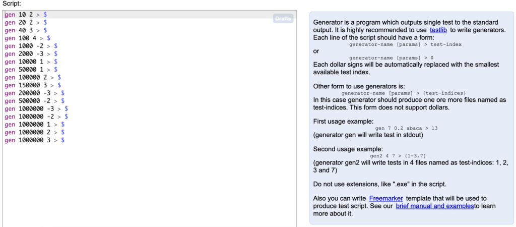
I have provided example of using randomization on the code snippets before this. These functions rnd.next, shuffle, and many more, uses randomization that will yield consistent result if given the same seed. To avoid repeating code in your generator files, you can make many adjustable aspects of your generators be your parameters of the files. As the image above suggest, it is creating TC for each call of the generator file, provided every value passed to the parameters and lastly the seed for each random method in that file to work with. With this one generator can serve many purpose if given different sets of values passed as parameters. In TCframe, the generators are not stored in files, instead in different method but in the same spec.cpp files, which means the usage of parameters become more intuitive.
To summarize, these are the main points to be addressed when creating TCs thorough enough to counter each unwanted solution of this problem that we studied.
| Solution Used | How to Stress Test Them |
|---|---|
| Naive DFS or BFS | Path and star graph |
| Lowest Common Ancestors | Make sure to create deep trees, the LCA of the two nodes is not near the root, maximize actual length of the path |
| Binary Lifting | Make sure the node pair’s depth of each query differ greatly, switch the node pair, the LCA is actually one of its nodes, the LCA is the root node |
| Range Update & Query Problem | Both extremes of focusing one query type, include long queries, and maximize type switching |
| Others | Use Randomization to ensure its correctness, keep in mind to calculate normal distributions if you want to rely on randomization |
Spoiler block
#include <bits/stdc++.h>
using namespace std;
#define ll long long

// I set the maxn to 1048576 since the constraint is 10**6 (1 million)
const ll maxn = (1<<20);

ll n, q;
ll nodeValues[maxn], sumToRoot[maxn]; // stores the values, and sumToRoot(i)
vector<ll> adjacencyList[maxn]; // stores the edges information

// For binary lifting, parent[i][j] stores the 2**j-th parent of node-i
ll parent[maxn][20], depth[maxn];
// Since about to do DFS, might as well flatten the tree
// Every node with a euler tour index inside the range subtreeRange[i] is a subtree of node-i
ll currentOrder = 0, subtreeRange[maxn][2];

// We need a method to get the direct parent for every node, if the root of the tree is 1
void dfs(ll node, ll from){
  // recursive searching from "node" but not through "from"
  subtreeRange[node][0] = currentOrder;
  for(ll i=0; i<adjacencyList[node].size(); i++){
    ll to = adjacencyList[node][i];
    if(to != from){
      // then "node" is the direct parent of "to", we can update information and do DFS
      parent[to][0] = node;
      depth[to] = depth[node] + 1;
      sumToRoot[to] = sumToRoot[node] + nodeValues[to]; // calculating sumToRoot
      currentOrder++; dfs(to, node); // recursive call, now node becomes from
    }
  }
  subtreeRange[node][1] = currentOrder;
}

// A method to calculate the 2**j-th parent of every node
void binaryLifting(){
  for(ll i=1; i<20; i++){
    for(ll j=1; j<=n; j++){
      parent[j][i] = parent[parent[j][i-1]][i-1];
    }
  }
}

//.A method to get Lowest Common Ancestor of node-x and node-y
ll getLCA(ll x, ll y){
  // make sure x is deeper in the tree than y
  if(depth[x] < depth[y]) swap(x, y);
  // lift x at max 20 times untill x is same depth with y
  for(ll i=19; i>=0; i--){
    if(depth[x] - (1<<i) >= depth[y]) x = parent[x][i];
  }
  // find the LCA by binary searching safe jump or unsafe jump
  for(ll i=19; i>=0; i--){
    if(parent[x][i] != parent[y][i]){
      x = parent[x][i]; y = parent[y][i];
    }
  }
  return x==y ? x : parent[x][0];
}

// For segment tree, segtree[i] stores sum of the range of nodes its responsible for

// segtree[maxn..2maxn-1] stores the value of arr[0..maxn]
// now arr[i] is the difference between sumToRoot of the i-th node in euler tour,
// and sumToRoot of (i-1)-th node in euler tour (0 if i=0)
// that way, sumToRoot of i-th node in euler tour is the sum of arr[0] + ... + arr[i]

// meanwhile the rest of segtree[1..maxn-1] is segtree[i] = segtree[2i] + segtree[2i+1]

ll segtree[maxn*2]; // initialized all 0

void update(ll idx, ll val){
  // add val to arr[i], this will update 20 nodes in the segtree
  for(ll i=idx+maxn; i>0; i/=2){
    segtree[i] += val;
  }
}

ll query(ll lower, ll higher){
  // returns arr[lower] + arr[lower+1] + ... + arr[higher-1] + arr[higher]
  lower += maxn; higher += maxn;
  ll result = 0;
  while(lower <= higher){
    if(lower%2 == 1) result += segtree[lower];
    lower = (lower+1)/2;
    if(higher%2 == 0) result += segtree[higher];
    higher = (higher-1)/2;
  }
  return result;
}

int main() {
  // inputting
  cin >> n >> q;
  for(ll i=1; i<=n; i++) cin >> nodeValues[i];
  for(ll i=1; i<n; i++){
    ll a, b; cin >> a >> b;
    adjacencyList[a].push_back(b);
    adjacencyList[b].push_back(a);
  }

  // usually, better to process the root node before DFS
  // but most initial values is already OK (all parent, depth, and currentOrder to be 0)
  sumToRoot[1] = nodeValues[1];
  dfs(1, 0);
  binaryLifting();

  // initialize the segtree
  for(ll i=1; i<=n; i++){
    update(subtreeRange[i][0], sumToRoot[i]);
    update(subtreeRange[i][0]+1, -sumToRoot[i]);
  }

  while(q--){
    ll type, a, b;
    cin >> type >> a >> b;
    if(type == 1){
      // change the value of node-a to b
      // update range of sumToRoot becomes update 2 points of arr
      update(subtreeRange[a][0], b - nodeValues[a]);
      update(subtreeRange[a][1]+1, nodeValues[a] - b);
      nodeValues[a] = b;
    }else{ // type == 2
      ll lca = getLCA(a, b);
      // The sum of values in a path a->b is
      // sumToRoot(a) + sumToRoot(b) - sumToRoot(lca) - sumToRoot(parent(lca))
      ll ans = query(0, subtreeRange[a][0]) + query(0, subtreeRange[b][0]);
      ans -= query(0, subtreeRange[lca][0]);
      if(lca > 1) ans -= query(0, subtreeRange[parent[lca][0]][0]);
      cout << ans << endl;
    }
  }
}
Above is my full solution to this problem that will pass any given TC that satisfies the problem constraint. Though I have not explained in detail, I also transformed the “Range Update Point Query” aspect to “Point Update Range Query” because that is easier to implement in my opinion. I did this by storing the adjacent-element-difference in the original array instead, and this makes the point query becomes the range sum of differences.
Afterwords
There are multiple kinds of problem I faced during my journey in this field, that I want to categorize depending on how the problem components are constructed, graded, and my experience working on them or solving them. Keep in mind these are an imperfect list based on my own experience, and I strongly believe there are more structured way to categorize CP Problems than this.
1. Partially-graded-problem with explicit subtasks
Subtasks are different sets of constraints that applies to the problem, usually sorted from easiest to solve, to hardest. The tests are grouped into these subtasks and the solver can actively see each constraints defined. This means we can get partial marks of this problem if our solution only solves the problem if the TC satisfies the easier subtasks. International Olympiad of Informatics (IOI) always uses this format in their problems.
2. Partially-graded-problem without giving explicit subtasks
This problem simply has many TCs that is unknown to the solver. Depending on how many TCs the solution solves, the score is computed according to each TC’s weight. Many interview problems usually use this approach to more accurately measure candidates’ capabilities.
3. Binary-graded-problem with deterministic solution
Binary-graded-problem is my way of saying the grade is either 1 meaning solved or get an accepted (AC) verdict, or 0 meaning unsolved, get a Wrong Answer (WA), Time Limit Exceeded (TLE), Memory Limit Exceeded (MLE), Runtime Error (RTE), or Compiler Error (CE). This is the most commonly encountered problem in CP, for example in well known websites such as CodeForces contests, Atcoder contests, TLX or even LeetCode.
4. Binary-graded-problem that has multiple solutions, output any
Same with the third point, but contains a checker in one of its problem setting components, as mentioned before. One example of this is one of my problem Bowling that you can freely try yourself! This is my first time writing an output-any problem so I find myself thinking the checker is actually more interesting than the solution. This is topic for another day…
5. Interactive problem
Same with the third point, but contains a communicator in one of its problem setting components, as mentioned before. One example of this is one of my problem Four Number Theorem from the same contest as the problem mentioned before. Once again a deep dive into this calls for another time.
6. Output only problem
Basically the solver submits only the output of their program after being executed in their own devices. Meaning the execution time is much larger than the usual time limit used in CP, from that in seconds, to that in hours.
As much as working on CP problem setting goes, it is similar to working on solving CP problem, in terms of arranging the building blocks you previously built each, to become a complete solution. In my short-but-continuously-learning experience of CP problem setting, the more I get familiar with each genre of the problem, the more I instinctively know which TCs are necessary to be generated in which problems. Even if I do not know what kind of solutions this TC fails.
Me personally, working on CP for a long time makes me always consider many edge cases or worst case scenario in the back of my mind, since I am trained to do so in a contest environment. I feel like this experience can potentially helps me write better purposed and structured tests for any business enterprise like Money Forward.
There is also this concept of pair programming in testing, which is to ensure the programmer writing a feature is different than the programmer writing the tests. Then the feature will undergo testing with similar feeling of a solver’s solution undergo jury’s TCs. I think this is quite interesting but I guess that is a topic for another day.
I hope this blog is greatly beneficial to all parties involved. As I am explaining every bit of this topic, I am quite enthusiastic. I am passionate to share this first-time-learning experience, since it was very mind-opening to me when I first learn about this. I am still doing CP for fun and CP Problem Setting for fun, as you can keep an eye on my activity in Codeforces-Kinon Atcoder-NonKi, TLX-nekogazaki_natsuho, or Leetcode-Kinon.
Happy coding!